Connected Components Matrix

Find The Number Of Islands Set 1 Using Dfs Geeksforgeeks
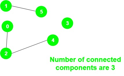
Program To Count Number Of Connected Components In An Undirected Graph Geeksforgeeks
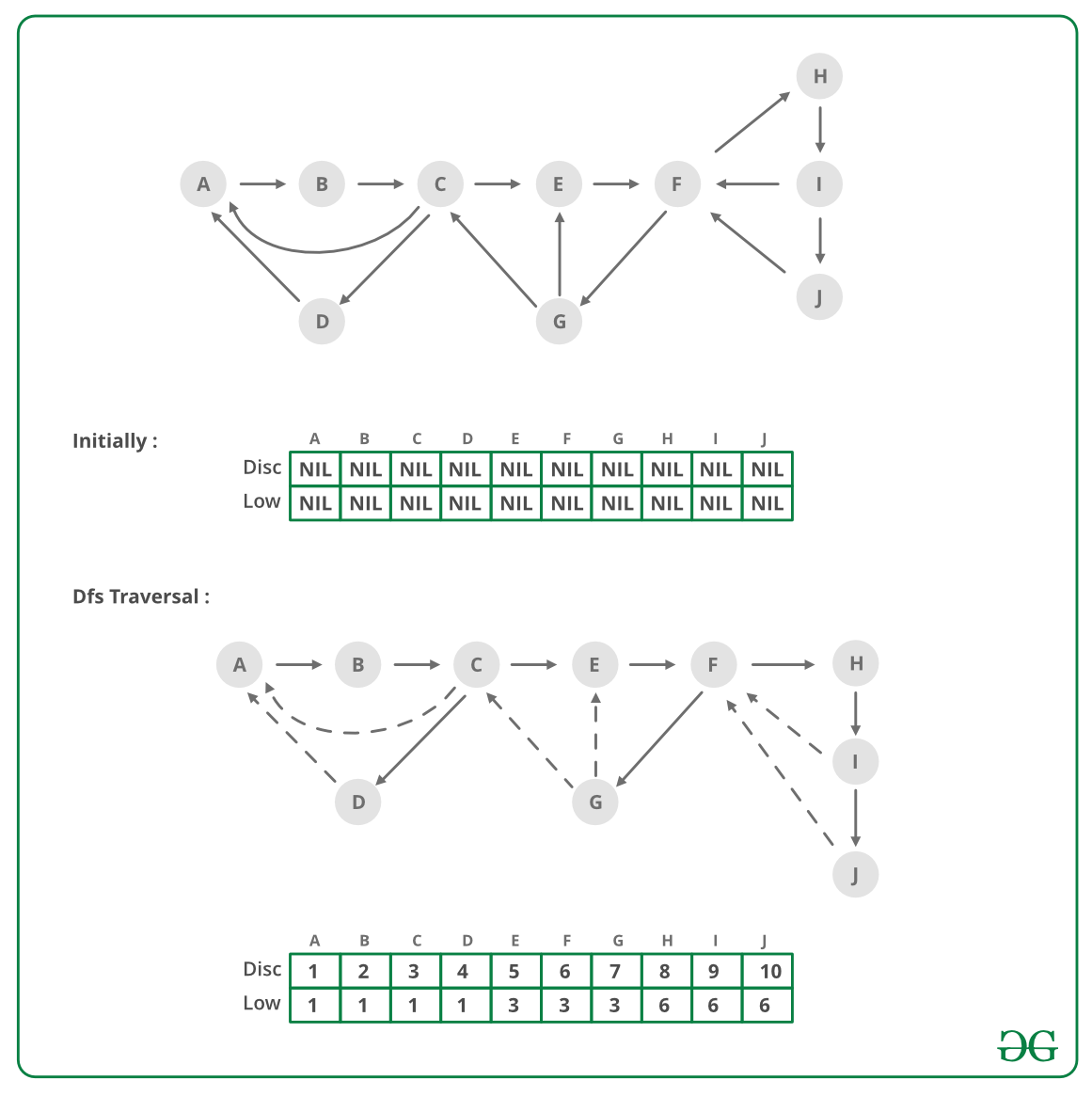
Tarjan S Algorithm To Find Strongly Connected Components Geeksforgeeks
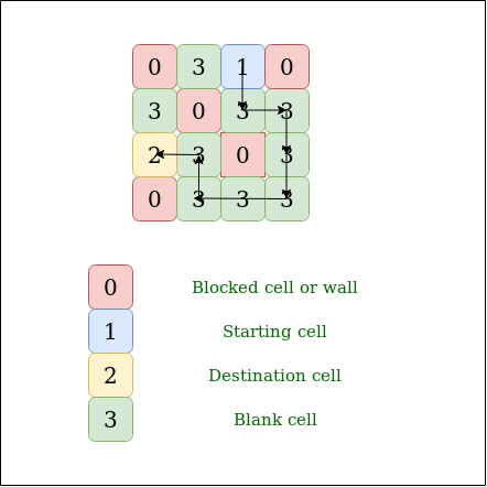
Find Whether There Is Path Between Two Cells In Matrix Geeksforgeeks

Adjacency Matrix From Wolfram Mathworld

An Adaptive Parallel Algorithm For Computing Connected Components

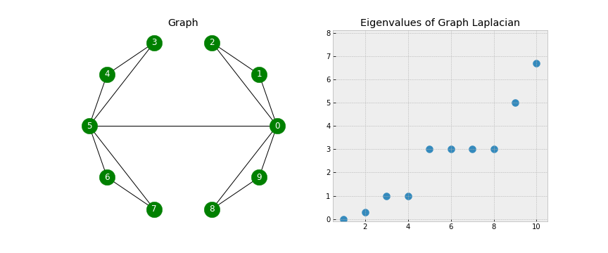
L is permutation similar to a block diagonal matrix.
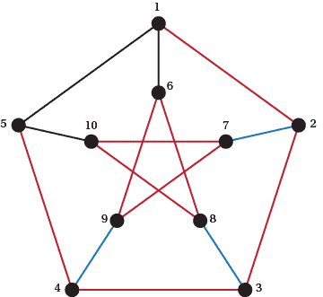
Connected components matrix.
An Introduction To Networks Math Insight

Global Stiffness Matrix An Overview Sciencedirect Topics
Spectral Clustering Foundation And Application By William Fleshman Towards Data Science
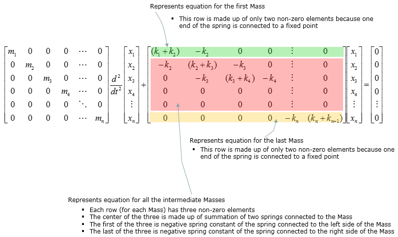
Differential Equation Modeling Spring And Mass Sharetechnote

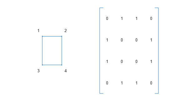
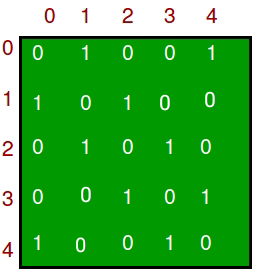
Adjacency Matrix An Overview Sciencedirect Topics

Graph And Its Representations Geeksforgeeks
Graphs And Matrices Matlab Simulink Example
Comparison Between Adjacency List And Adjacency Matrix Representation Of Graph Geeksforgeeks
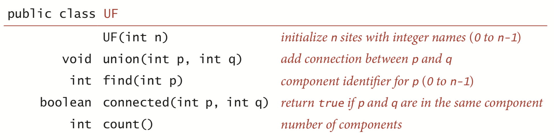
Case Study Union Find
Algorithms For Generating All Possible Spanning Trees Of A Simple Undirected Connected Graph An Extensive Review Springerlink

4 Components Of Successful Change In Organization Jpg 1824 1794 Change Management Change Leadership Change Management Models

Connected Subgraph An Overview Sciencedirect Topics

One Dimensional Array An Overview Sciencedirect Topics
From Theory To Practice Representing Graphs By Vaidehi Joshi Basecs Medium

Information Systems Strategy Matrix System Physics Networking

Graph Theory 17 Adjacency Matrix Of A Directed Connected Graph Youtube

Statistical Connectomics Sciencedirect

Rotated Component Matrix Of Factor Analysis In Spss Is Not Coming As Expected Can Some One Tell Me Why
Https Encrypted Tbn0 Gstatic Com Images Q Tbn 3aand9gcs8eg6g6ckt2swyejkggggbradpz1cmpjnz3762y7 Dpxldiwon Usqp Cau
Tssn Crossbar Switching Tutorialspoint
Graphs In Java Baeldung

Butler Matrix Wikipedia

Element Stiffness Matrix An Overview Sciencedirect Topics
Answers To Questions
Source : pinterest.com
